An introduction to Deep Adaptive Design (DAD)

In the blog post, I introduce Deep Adaptive Design (DAD), a popular computational approach for implementing Bayesian Optimal Experimental Design. This post includes a whistle stop tour of the core concepts of BED, neural networks and embeddings, written with statisticians in mind who are new to the world of machine learning (like me)!

A whistle stop tour of Bayesian Experimental Design

Bayesian Experimental Design (BED) formalises what it means for an experiment to be optimal. If you were running a sequential experiment, it would be human nature to choose the next experiment based on how relevant its outcome could be for the task at hand and on where our uncertainty is greatest. In essence, BED replicates the intuitive approach we as humans would make when deciding what experiment to run, though to consider this problem statistically, beliefs are informed by priors on statistical models and uncertainty is statistically propagated across the potentially true model parameters and potential outcomes we may observe.

One of the most common approaches to conducting an optimal experiment is by considering an experiment’s expected information gain (EIG). An experiment that maximises EIG is expected to produce the strongest update to our beliefs when we observe its outcome.

I like to explain BED in terms of Wordle. All Wordle users have the same goal - to identify the word of the day with as few guesses as possible. We wish to learn what the secret word of the day is, which in statistical terms can be translated to learning about an unknown parameter \(\theta\) (the secret word in this case). As Wordle players, we are in control of the designs \(\xi\) we choose which, in this case, represent the potential 5-letter word choices we can make. Once we have guessed a word, we observe an outcome \(y\) and then guess a new five-letter word using this guess. For Wordle, \(y\) is the coloured code representing how many letters of the secret word we correctly identified and their location in the word.

At the very start of playing Wordle, we wish to choose the word which maximises the EIG across all potential 5-letter words \(\xi \in \Xi\) we can guess. The EIG for each word at the start of Wordle can be written as,

To understand this formula, suppose we wish to quantitatively evaluate the benefit of guessing the word ‘ADIEU’ for today’s Wordle.

Inner integral: Suppose we guessed ‘ADIEU’ and observed outcome ⬜⬜⬜🟨⬜. In this case, we know only the letter E from ADIEU is in the secret word, though it is not the fourth letter. To evaluate how good our guess of ‘ADIEU’ was having observed outcome ⬜⬜⬜🟨⬜, we need to evaluate how much we learnt across all potential secret words $\theta \in \Theta$ (around 2,300 options). Thus, we first propagate our uncertainty across all potential parameter options $\theta$ we may see. For example, this guess certainly means we no longer suspect ‘BUZZY’ of being the secret word, but it hasn’t helped us learn whether the secret word is either ‘WHOLE’ or ‘PROSE’. This inner integral helps us mathematically quantify this learning.

Inner integral: The outer integral recognises that we cannot observe outcome ⬜⬜⬜🟨⬜ without choosing ADIEU as a guess to start with. This goes against the whole point of the challenge, we want to know if ‘ADIEU’ is a good word to guess before wasting a Wordle turn on it. In this case we must also propagate our uncertainty once more over all the potential colour patterns we may see for the word ‘ADIEU’. For example, as ‘ADIEU’ has lots of vowels, we expect the colour pattern to have more yellows and greens compared to a more unusual word like ‘FLUFF’ which, with its repeated F’s, is less likely to share many letters with the secret word.

Accordingly, the best first guess for Wordle will be \(\xi^* = \arg \max_{\xi \in \Xi} EIG_\theta(\xi).\)

Whilst it is not notationally challenging to write the objective down for the best Wordle word, computationally it is a different story. Maximising the EIG is a doubly intractable objective, which introduces a huge computational bottleneck for the real time deployment of experiments wishing to leverage BED. This sets the scene for DAD (Deep Amortised Design).

Amortising BED

The idea of amortising processes has come up many times since starting my postdoc. In the previous section we discussed the case where at each step of an experiment, a doubly intractable objective must be optimised, with a huge computational cost. Amortisation considers an approach where rather than evaluating this objective at each data acquisition step during the live experiment, we instead train a strategy upfront, before deployment (active use). By doing so, model training is completed before the experiment begins. Thus, whilst it make take a while to train the model before deployment, once the experiment is underway, decision-making on which experiment to run next can be made almost instantaneously.

For DAD, this strategy means that a design policy \(\pi\) (Neural Network) is trained to acquire data intelligently before the experiment is even run so that, once the experiment commences, decision-making is as simple as completing one forward pass (one model evaluation) of the network to recommend the next experiment using the history of previous experiments.

As the neural network is trained before the experiment has even been run, the design policy is trained on synthetic data using the known prior and likelihood of the model. Then, after model training, the design policy can be used in real time by practitioners for almost instantaneous real-time for decision-making, bypassing the computationally expensive necessity to compute the doubly intractable objective (1) to compute the EIG.

Neural Networks

Whilst neural Networks have always struck me as mystical black boxes, broadly speaking their specific approach to model fitting is somewhat similar to more statistically-minded approaches such as ordinary least squares estimator for linear regression. It is more so their intricate architecture, rather than their broader methodology, which differs.

Like any statsitical model, with a neural network you have a number of inputs which you wish to use to predict some output. Similarly to a linear regression, a neural network takes these inputs and finds a relationship to map the inputs to an output. The exact relationship between inputs and outputs is formed in hidden layers of the neural network.

Consider a simple neural network with \(L\) layers which looks something like,

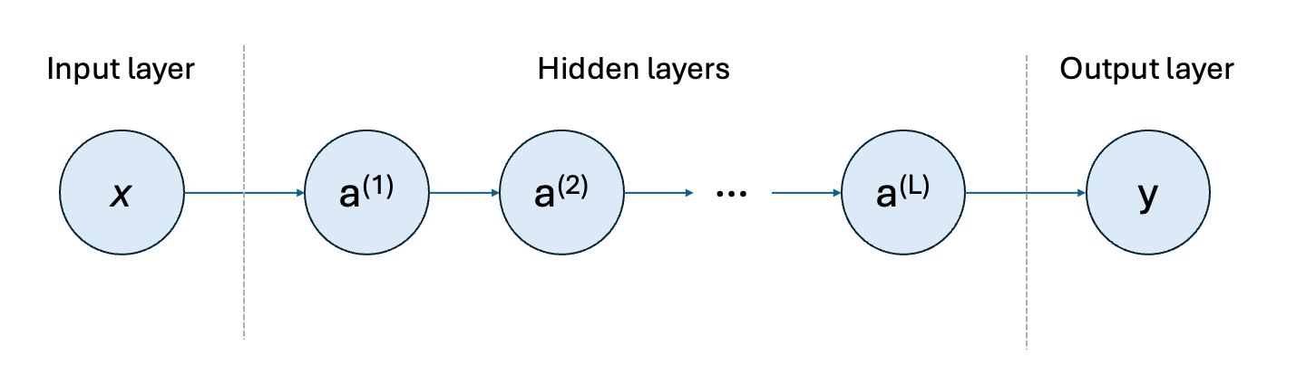
We start with our raw inputs \(x\). These raw inputs are linearly transformed given a weight \(w^{(1)}\) and bias \(b^{(1)}\) such that \(z^{(1)} = w^{(1)}x + b^{(1)}\). \(z^{(1)}\) is then transformed using a non-linear transformation \(\sigma^{(1)}\) such that \(a^{(1)} = \sigma^{(1)}(z^{(1)})\). Exemplar functions \(\sigma^{(1)}\) can include sigmoid() or tanh() functions.

Now at the second layer, the activation function consists of a non-linear transformation of a linear transformation of the proceeding activation function. For example, \(a^{(2)} = \sigma^{(2)}(w^{(2)}a^{(1)} + b^{(2)}) = \sigma^{(2)}(w^{(2)}\sigma^{(1)}(w^{(1)}x + b^{(1)}) + b^{(2)})\). A third layer has an activation function which is a function of the proceeding activation function from the second layer and so on. By adding more layers to the neural network, we increase its depth. All these nodes between the inputs and final predicted layers are called hidden layers. Once we have computed the activation function for the final layer $L$, there are by now many parameters (weights and biases) associated with the predictive task.

Now we have to evaluate the predictive performance of the neural network. To do so, when we train the neural network, we compare our network’s prediction to the true outcome using a loss, such as the sum of squared residuals used in linear regression.

A model which uses the inputs and predicts the outcomes perfectly would have zero loss and as such, we wish to train our neural network to minimise the loss as much as possible. Accordingly, during training, we iteratively tune the neural network’s parameters (weights and biases) in the hope that by tuning these parameters the network will perform better at a future predictive task. We do this by backpropagating the neural network. This just means we differentiate the loss with respect to all the parameters. Given the graphical nature of the network, with all weights and biases nested in the final activation function, this can be done using the chain rule. By differentiating, we can identify the rate at which each parameter contributes to the overall loss and as such, weights and biases can be tuned to reduce this loss and thus improve model prediction. Once the network has been backpropagated and gradients for each parameter identified, the network can be optimised and parameters tuned to reduce the loss.

This process of making a forward pass of the model (running the model for new input data), comparing the prediction to the true outcome using a loss, backpropagating, and optimising the network is repeated over and over again using training data until the model is sufficiently trained and ready for deployment.

Whilst this section has introduced neural networks considering an example with a single node per layer, we can increase the width of the network by adding multiple nodes per layer. Intuitively, this does not add much additional complication, with the main change being that the activation for each node at a certain layer is now an aggregate of the weights and biases associated with the nodes in the previous layer.

import torch 
import torch.nn as nn
import os

Embeddings

In a neural network, you may not wish to input raw data in the input layer. Rather you may wish to use a representation of the data using an embedding. Embeddings can be used to transform complex data (such as audio or image data) into lower-dimensional objects for use in a machine learning models. In this way, embeddings can learn the important relationships of the higher dimensional space whilst its lower dimensional representation is easier to work with and more computationally efficient. Alternatively, as per the code below, embeddings can also be used to map lower-dimensional raw data into a higher-dimensional representation. This may help models recognise more granular nuances in the data.

These embeddings can be learnt using neural networks. For example, in the code below for a neural network called encoder, we take some raw data of dimension 2, have a single hidden layer of 128 nodes and output a new representation of the raw data with dimension 8. This eight-dimensional representation is used as the input to some model with a specific prediction task encoded into its loss. As such, when the neural backpropagates using this loss, the weights and biases associated with this embedding are tuned to ensure a more effective embedding can be utilised.

class encoder(nn.Module):
    def __init__(self, num_inputs = 2, num_hidden=128, num_outputs=8):
        super().__init__()
        self.linear1=nn.Linear(num_inputs, num_hidden)
        self.act_fn=nn.ReLU()
        self.linear2=nn.Linear(num_hidden, num_outputs)

    def forward(self, x):
        x=self.linear1(x)
        x=self.act_fn(x)
        x=self.linear2(x)
        return x

Exemplar problem

Consider a scenario where we wish to identify the location of a signal source somewhere in one-dimensional space. In this example, we can choose points in space and estimate the signal intensity at each one. Suppose we can complete $T$ experiments and by the end of the 15th experiment, we want to have identified the location of the source \(\theta\) as precisely as possible.

To use DAD in this scenario we need a model for the signal strength. At location \(\xi\), if the source of the signal is \(\theta\) the signal strength is known to be, \(\mu(\theta, \xi) = 10^{-1} + \frac{1}{10^{-4} + || \theta - \xi||^2}.\)

def signal(theta_0, xi, alpha = torch.tensor([1]), b = torch.tensor([10**-1]), m = torch.tensor([10**-4])):
    return b + (alpha)/(m + (theta_0-xi)**2)

Our observations are subject to some noise and as such the likelihood of observing signal strength \(y\) conditional on the location of experiment \(\xi\) and true source location \(\theta\) can be written as, \(y \mid \theta, \xi \sim \text{LogNormal}(\log(\mu(\theta, \xi), 0.5)).\) We consider the following prior on the source location, \(\theta \sim N(0,1)\).

Implementation

DAD is trained before data is even seen using synthetic data coming from the prior. In this way, the neural network can be trained to select new data points using previous history before the experiment even commences. Then at deployment, decision-making on which experiment to conduct next is made by the trained neural network almost instantaneously by doing on forward pass of the model, rather than by completing a computationally burdensome Monte Carlo estimate for the doubly intractable integral.

The trained neural network \(\pi\) is the design policy. Whilst the policy could be trained to take in all the history of experiments so far \(h_t = \{(\xi_1, y_1), (\xi_t, y_t)\}\), instead in this example it takes in a representation of this experiment and outputs the next recommended experiment \(\xi_{t+1}\). This is done using the encoder code we presented in the section on embeddings.

Our encoder starts with two dimensions for \((\xi_t, y_t)\) at fixed experiment $t$ and transforms it to an 8 dimensional representation. The sum of this representation across all experiments completed so far is then fed into another neural network called emitter which takes this 8 dimensional representation, feeds it into a hidden layer of 2 nodes and outputs a new location to test $\xi_t$ with a single dimension, summarised notationally as \(\pi(h_{t-1})\).

class emitter(nn.Module):
    def __init__(self, num_inputs=8, num_hidden=2, num_outputs=1):
        super().__init__()
        self.linear1=nn.Linear(num_inputs, num_hidden)
        self.linear2=nn.Linear(num_hidden, num_outputs)

    def forward(self, x):
        x=self.linear1(x)
        x=self.linear2(x)
        return x

The ‘encoder’ and ‘emitter’ neural networks combine together to make the design policy neural network.

class Policy(nn.Module):
    def __init__(self, encoder, emitter):
        super().__init__()
        self.encoder = encoder
        self.emitter = emitter
        self.norm = nn.LayerNorm(encoder.linear2.out_features)

    def forward(self, history):
        B, T, D = history.shape
        
        if T==0:
            z = history.new_full((B, self.encoder.linear2.out_features), 0)
        else:
            encoded = self.encoder(history.reshape(B*T, D))
            encoded = encoded.reshape(B, T, -1)
            z=encoded.sum(dim=1)
            z = self.norm(z)
        xi_t = self.emitter(z)
        return xi_t

Now we have defined our neural network we need to train it using synthetic data in order to recommend good experiments which are maximising our EIG. We create a set of training data (\(L\) complete experiment rollouts (full experiments)) which we wish to use for one optimisation of the neural network as follows:

For \(l = 1,...,L\):
      Sample the location of a signal \(\theta_0 \sim N(0,1)\)
      For \(t = 1,...,T\):
            Compute the next design \(\xi_t = \pi(h_{t-1})\)
            Sample \(y_t \sim p(y \mid \theta_0, \xi_t)\)
            Set \(h_t = \{(\xi_1, y_1), ..., (\xi_t, y_t)\}\).

Now we have completed \(L\) full, synthetic experiments, we can estimate the average EIG for this policy \(\pi\). Whilst neural networks usually wish to minimise some predictive loss, for this use case we wish to maximise the EIG of the policy $\pi$. As such, our loss in this case is the negative estimated EIG. To backpropagate using this loss, we need to ensure that any loss we choose is both computable and differentiable. As the EIG itself is doubly intractable, a contrastive bound acting as a lower bound of the EIG is used as the loss rather than the EIG itself for computational reasons. Thus, if we can maximise this lower bound of the EIG, we can tune our policy’s parameters toward a data acquisition policy which better maximises the EIG of the experiments we undertake. More details of the exact approximation can be found in the original paper, with code provided here just for completeness.

def log_likelihood(y_T, theta, xi_T):
    y_T = y_T.unsqueeze(1)
    xi_T = xi_T.unsqueeze(1)
    scale = torch.tensor(0.5, device=theta.device, dtype=theta.dtype)
    dist = torch.distributions.LogNormal(loc = torch.log(signal(theta, xi_T)), scale = scale)
    return dist.log_prob(y_T).sum(dim=-1)

def gL_batch(theta_0, history_B, L):
    B = theta_0.shape[0]
    log_y_T = history_B[:, :, 1]
    y_T = log_y_T.exp()
    xi_T = history_B[:,:,0]

    theta_l = torch.distributions.Normal(loc = 0, scale = 1).rsample((B,L,1))
    theta_0_L = torch.cat([theta_0.unsqueeze(1), theta_l], dim=1)
    log_liks = log_likelihood(y_T, theta_0_L, xi_T)
    true_log_lik = log_liks[:, 0]
    gL = (true_log_lik- torch.logsumexp(log_liks, dim=1)+ torch.log(torch.tensor(L + 1)))
    return gL.mean()

Accordingly, when \(L\) full, synthetic experiments have been undertaken, we approximate the total EIG associated with policy \(\pi\), backpropagate the neural network and subsequently tune our parameters with the aim of improving upon the average total EIG associated with our design policy by training the model toward a more negative loss. We then repeat this process, running another \(L\) experiments, backpropagating, and tuning parameters once more to improve the neural network. As a result, the design policy is continually updated and refined to select increasingly informative locations at which to detect the signal in an effort to identify its true source.

The code to run DAD for this example is found below.

B = 1000
L = 1000
T = 15

gradient_steps = 4000
annealing_frequency = 1000
gamma = 0.95
betas = (0.8, 0.998)

policy = Policy(encoder(), emitter())
optimiser=torch.optim.Adam(policy.parameters(), lr=0.0001, betas=betas)


scheduler = torch.optim.lr_scheduler.StepLR(optimiser,step_size=annealing_frequency,gamma=gamma,)
save_dir = "results"
loss_history = []

for step in range(gradient_steps):
    optimiser.zero_grad()
    theta_0 = torch.distributions.Normal(loc = 0, scale = 1).rsample((B,1))
    history = torch.empty(B, 0, 2)
    for t in range(T):
        xi_t = policy(history.float())
        mean = torch.log(signal(theta_0, xi_t))
        log_y_t = torch.distributions.Normal(loc = mean, scale = torch.tensor(0.5, dtype=torch.float32)).rsample()
        new_pair = torch.stack([xi_t, log_y_t], dim=2)
        history = torch.cat([history, new_pair], dim=1)
    loss = -gL_batch(theta_0, history,L)
    wandb.log({"loss": loss.item(), "step": step})
    loss_history.append(loss.item())
    print(loss)
    torch.save({
    "step": step,
    "optimiser_state_dict": optimiser.state_dict(),
    "policy_state_dict": policy.state_dict(),
    "loss": loss.item(),
    "loss_history": loss_history,
    }, os.path.join(save_dir, f"checkpoint_step_{step}.pt"))
    
    
    loss.backward()
    torch.nn.utils.clip_grad_norm_(policy.parameters(), max_norm=1.0)
    optimiser.step()
    scheduler.step()

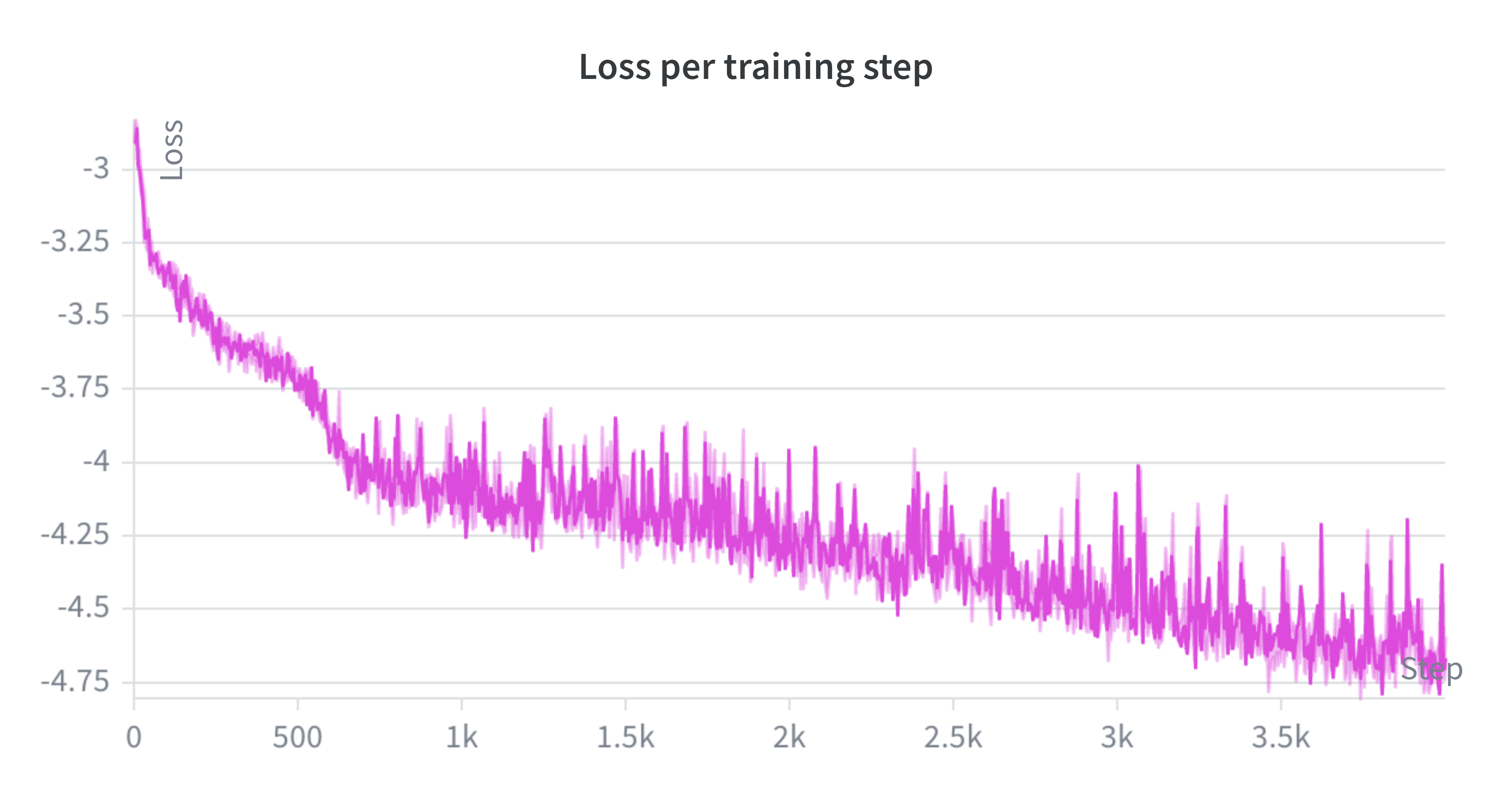
Below I share a figure showing the loss (negative contrastive lower bound) of the EIG for 4,000 policy design updates for DAD. You can see how, in general, every time I backpropagate and tune the neural network (recorded on the x-axis) the total EIG associated with the design policy generally seems to improve (with the negative EIG becoming more negative). As such, each subsequent neural network generally recommends new experiments which are even better at maximising the overall EIG of the experiment. After training the model across 4,000 optimisations (or once training budget has been depleted) this design policy may now be ready for deployment and used in real time for data gathering.